Introduction to parallel & distributed algorithms

Contents
1.	Parallel & distributed models 1.1. Parallel computing 1.2. Distributed computing
2.	Parallel scan 2.1. Adding array entries 2.2. Generalizing to parallel scan 2.3. Counting initial 1's 2.4. Evaluating a polynomial
3.	Parallel prefix scan 3.1. The prefix scan algorithm 3.2. Filtering an array 3.3. Adding big integers
4.	Sorting 4.1. Merging 4.2. Mergesort
5.	Hardness of parallelization
	Review questions Solutions to review questions Exercises
	References

by Carl Burch, Hendrix College, August 2009

This was written as a unit for an introductory algorithms course. It's material that often doesn't appear in textbooks for such courses, which is a pity because distributed algorithms is an important topic in today's world.

PDF version available

Introduction to parallel & distributed algorithms by Carl Burch is licensed under a Creative Commons Attribution-Share Alike 3.0 United States License.
Based on a work at www.cburch.com/books/distalg/.

Classically, algorithm designers assume a computer with only one processing element; the algorithms they design are said to be sequential, since the algorithms' steps must be performed in a particular sequence, one after another. But today's computers often have multiple processors, each of which performs its own sequence of steps. Even basic desktop computers often have multicore processors that include a handful of processing elements. But also significant are vast clusters of computers, such as those used by the Department of Defense to simulate nuclear explosions and by Google to process search engine queries. An example is the Roadrunner system at Los Alamos National Laboratory. As of 2009, it has 129,600 processors and is ranked as the world's fastest supercomputer.

Suppose we're working with such a real-world multiprocessor system. Inevitably, we'll run into some problem that we want it to solve. Letting T represent the amount of time that a single processor takes to solve this problem, we would hope to develop an algorithm that takes T / p time on a p-processor system. (We'll invariably use the variable p to represent the number of processors in our system.) In reality, this will rarely be possible to achieve entirely: The processors will almost always need to spend some time coordinating their work, which will lead to a penalty.

Sometimes such a near-optimal speedup is easy to achieve. Suppose, for instance, that we have an array of integers, and we want to display all the negative integers in the array. We can divide the array into equal-sized segments, one segment for each processor, and each processor can display all the negative integers in its segment. The sequential algorithm would take O(n) time. In our multiprocessor algorithm each processor handles an array segment with at most ⌈n / p⌉ elements, so processing the whole array takes O(n / p) time.

But there are some problems where it is hard to imagine how to use multiple processors to speed up the processing time. An example of this is determining the depth-first search order of a graph: It seems that any algorithm will be forced to process a child only after its parent, so if the graph's height is something like n / 2, it will necessarily take O(n) time. This seems like an inherently sequential problem. And, indeed, it has proven to be so, as we'll see in Section 5.

Or consider the problem where we're given two integer arrays representing very large numbers (where a[0] contains the 1's digit, a[1] contains the 10's digit, and so on), and we want to compute a new array containing the sum of the two numbers. From grade school, you know a sequential algorithm to do this that takes O(n) time. We can't easily adapt this algorithm to use many processors, though: In processing each segment of the arrays, we need to know whether there is a carry from the preceding segments. Thus, this problem too seems inherently sequential. But in this case our intuition has failed us: We'll see in Section 3.3 that in fact there is an algorithm that can add two such big-integers in O(n / p + log p) time.

As with adding big-integers, some very simple problems that we consider hardly worth studying in single-processor systems become more interesting in the multiprocessor context. This introduction will pay particularly close attention to algorithms that deal with arrays of numbers. We'll begin in Section 1 by first presenting more formal models of parallel and distributed systems. Then in Section 2 we'll look at the particularly simple problem of adding all the numbers of an array, a problem that can be generalized to parallel scan, which can be applied to other situations as well. In Section 3, we'll look at a closely related algorithm called parallel prefix scan, and again we'll look at several of its applications. Section 4 will look at the problem of sorting an array on a multiprocessor system, while Section 5 will discuss how complexity theory can be used to argue that problems are indeed inherently sequential.

1. Parallel & distributed models

Multiprocessor systems come in many different flavors, but there are two basic categories: parallel computers and distributed computers. These two terms are used with some overlap, but usually a parallel system is one in which the processors are closely connected, while a distributed system has processors that are more independent of each other.

1.1. Parallel computing

In a parallel computer, the processors are closely connected. Frequently, all processors share the same memory, and the processors communicate by accessing this shared memory. Examples of parallel computers include the multicore processors found in many computers today (even cheap ones), as well as many graphics processing units (GPUs).

As an example of code for a shared-memory computer, below is a Java fragment intended to find the sum of all the elements in a long array. Variables whose name begin with my_ are specific to each processor; this might be implemented by storing these variables in individual processors' registers. The code fragment assumes that a variable array has already been set up with the numbers we want to add and that there is a variable procs that indicates how many processors our system has. In addition, we assume each register has its own my_pid variable, which stores that processor's own processor ID, a unique number between 0 and procs − 1.

// 1. Determine where processor's segment is and add up numbers in segment. count = array.length / procs; my_start = my_pid * count; my_total = array[my_start]; for(my_i = 1; my_i < count; my_i++) my_total += array[my_start + my_i]; // 2. Store subtotal into shared array, then add up the subtotals. subtotals[my_pid] = my_total; // line A in remarks below my_total = subtotals[0]; // line B in remarks below for(my_i = 1; my_i < procs; my_i++) { my_total += subtotals[my_i]; // line C in remarks below } // 3. If array.length isn't a multiple of procs, then total will exclude some // elements at the array's end. Add these last elements in now. for(my_i = procs * count; my_i < array.length; my_i++) my_total += array[my_i];

Here, we first divide the array into segments of length count, and each processor adds up the elements within its segment, placing that into its variable my_total. We write this variable into shared memory in line A so that all processors can read it; then we go through this shared array of subtotals to find the total of the subtotals. The last step is to take care of any numbers that may have been excluded by trying to divide the array into p equally-sized segments.

Synchronization

An important detail in the above shared-memory program is that each processor must complete line A before any other processor tries to use that saved value in line B or line C. One way of ensuring this is to build the computer so that all processors share the same program counter as they step through identical programs. In such a system, all processors would execute line A simultaneously. Though it works, this shared-program-counter approach is quite rare because it can be difficult to write a program so that all processors work identically, and because we often want different processors to perform different tasks.

The more common approach is to allow each processor to execute at its own pace, giving programmers the responsibility to include code enforcing dependencies between processors' work. In our example above, we would add code between line A and line B to enforce the restriction that all processors complete line A before any proceed to line B and line C. If we were using Java's built-in features for supporting such synchronization between threads, we could accomplish this by introducing a new shared variable number_saved whose value starts out at 0. The code following line A would be as follows.

synchronized(subtotals) { number_saved++; if(number_saved == procs) subtotals.notifyAll(); while(number_saved < procs) { try { subtotals.wait(); } catch(InterruptedException e) { } } }

Studying specific synchronization constructs such as those in Java is beyond this tutorial's scope. But even if you're not familiar with such constructs, you might be able to guess what the above represents: Each processor increments the shared counter and then waits until it receives a signal. The last processor to increment the counter sends a signal that awakens all the others to continue forward to line B.

Shared memory access

Another important design constraint in a shared-memory system is how programs are allowed to access the same memory address simultaneously. There are three basic approches.

CRCW: Concurrent Read, Concurrent Write. Simultaneous reads and writes are allowed to a memory cell. The model must indicate how simultaneous writes are handled.
- Common Write: If processors write simultaneously, they must write same value.
- Priority Write: Processors have priority order, and the highest-priority processor's write wins in case of conflict.
- Arbitrary Write: In case of conflict, one of the requested writes will succeed. But the outcome is not predictable, and the program must work regardless of which processor wins.
- Combining Write: Simultaneous writes are combined with some function, such as adding values together.
CREW: Concurrent Read, Exclusive Write. Here different processors are allowed to read the same memory cell simultaneously, but we must write our program so that only one processor can write to any memory cell at a time.
EREW: Exclusive Read, Exclusive Write. The program must be written so that no memory cell is accessed simultaneously in any way.
ERCW: Exclusive Read, Concurrent Write. There is no reason to consider this possibility.

In our array-totaling example, we used a Common-Write CRCW model. All processors write to the count variable, but they all write an identical value to it. This write, though, is the only concurrent write, and the program would work just as well with count changed to my_count. In this case, our program would fit into the more restrictive CREW model.

1.2. Distributed computing

A distributed system is one in which the processors are less strongly connected. A typical distributed system consists of many independent computers in the same room, attached via network connections. Such an arrangement is often called a cluster.

In a distributed system, each processor has its own independent memory. This precludes using shared memory for communicating. Processors instead communicate by sending messages. In a cluster, these messages are sent via the network. Though message passing is much slower than shared memory, it scales better for many processors, and it is cheaper. Plus programming such a system is arguably easier than programming for a shared-memory system, since the synchronization involved in waiting to receive a message is more intuitive. Thus, most large systems today use message passing for interprocessor communication.

From now on, we'll be working with a message-passing system implemented using the following two functions.

void send(int dst_pid, int data): Sends a message containing the integer data to the processor whose ID is dst_pid. Note that the function's return may be delayed until the receiving processor requests to receive the data — though the message might instead be buffered so that the function can return immediately.
int receive(int src_pid): Waits until the processor whose ID is src_pid sends a message and returns the integer in that message. This is called a blocking receive. Some systems also support a non-blocking receive, which returns immediately if the processor hasn't yet sent a message. Another variation is a receive that allows a program to receive the first message sent by any processor. However, in our model, the call will always wait until it receives a message (unless there is already a message waiting to be sent), and the source processor's ID must always be specified.

To demonstrate how to program in this model, we return to our example of adding all the numbers in an array. We imagine that each processor already has its segment of the array in its memory, called segment. The variable procs holds the number of processors in the system, and pid holds the processor's ID (a unique integer between 0 and procs − 1, as before).

total = segment[0]; for(i = 1; i < segment.length; i++) total += segment[i]; if(pid > 0) { // each processor but 0 sends its total to processor 0 send(0, total); } else { // processor 0 adds all these totals up for(int k = 1; k < procs; k++) total += receive(k); }

This code says that each processor should first add the elements of its segment. Then each processor except processor 0 should send its total to processor 0. Processor 0 waits to receive each of these messages in succession, adding the total of that processor's segment into its total. By the end, processor 0 will have the total of all segments.

In a large distributed system, this approach would be flawed since inevitably some processors would break, often due to the failure of some equipment such as a hard disk or power supply. We'll ignore this issue here, but it is an important issue when writing programs for large distributed systems in real life.

2. Parallel scan

Summing the elements of an n-element array takes O(n) time on a single processor. Thus, we'd hope to find an algorithm for a p-processor system that takes O(n / p) time. In this section, we'll work on developing a good algorithm for this problem, then we'll see that this algorithm can be generalized to apply to many other problems where, if we were to write a program to solve it on a single-processor system, the program would consist basically of a single loop stepping through an array.

2.1. Adding array entries

So how does our program of Section 1.2 do? Well, the first loop to add the numbers in the segment takes each processor O(n / p) time, as we would like. But then processor 0 must perform its loop to receive the subtotals from each of the p − 1 other processors; this loop takes O(p) time. So the total time taken is O(n / p + p) — a bit more than the O(n / p) time we hoped for.

(In distributed systems, the cost of communication can be quite large relative to computation, and so it sometimes pays to analyze communication time without considering the time for computation. The first loop to add the numbers in the segment takes no communication, but processor 0 must wait for p − 1 messages, so our algorithm here takes O(p) time for communication. In this introduction, though, we'll analyze the overall computation time.)

Is the extra + p in this time bound something worth worrying about? For a small system where p is rather small, it's not a big deal. But if p is something like n^0.8, then it's pretty notable: We'd be hoping for something that takes O(n / n^0.8) = O(n^0.2) time, but we end up with an algorithm that actually takes O(n^0.8) time.

Here's an interesting alternative implementation that avoids the second loop.

total = segment[0]; for(i = 1; i < segment.length; i++) total += segment[i]; if(pid < procs - 1) total += receive(pid + 1); if(pid > 0) send(pid - 1, total);

Because there's no loop, you might be inclined to think that this takes O(n / p) time. But we need to remember that receive is a blocking call, which can involve waiting. As a result, we need to think through how the communication works. In this fragment, all processors except the last attempt to receive a message from the following processor. But only processor p − 1 skips over the receive and sends a message to its predecessor, p − 2. Processor p − 2 receives that message, adds it into its total, and then sends that to processor p − 3. Thus our totals cascade down until they reach processor 0, which does not attempt to send its total anywhere. The depth of this cascade is p − 1, so in fact this fragment takes just as much time as before, O(n / p + p).

Can we do any better? Well, yes, we can: After all, in our examples so far, we've had only one addition of subtotals at a time. A simple improvement is to divide the processors into pairs, and one processor of each pair adds its partner's subtotal into its own. Since all these p / 2 additions happen simultaneously, this takes O(1) time — and we're left with half as many subtotals to sum together as before. We repeat this process of pairing off the remaining processors, each time halving how many subtotals remain to add together. The following diagram illustrates this. (The blue numbers indicate processor IDs.)

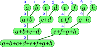
Thus, in the first round, processor 1 sends its total to processor 0, processor 3 to processor 2, and so on. The p / 2 receiving processors all do their work simultaneously. In the next round, processor 2 sends its total to processor 0, processor 6 to processor 4, and so on, leaving us with p / 4 sums, which again can all be computed simultaneously. After only ⌈log₂ p⌉ rounds, processor 0 will have the sum of all elements.

The code to accomplish this is below. The first part is identical; the second looks a bit tricky, but it's just bookkeeping to get the messages passed as in the above diagram.

total = segment[0]; for(i = 1; i < segment.length; i++) total += segment[i]; for(int k = 1; k < procs; k *= 2) { if((pid & k) != 0) { send(pid - k, total); break; } else if(pid + k < p) { total += receive(pid + k); } }

This takes O(n / p + log p) time, which is as good a bound as we're going to get.

(A practical detail that's beyond the scope of this work is how to design a cluster so that it can indeed handle sending p / 2 messages all at once. A poorly designed network between the processors, such as one built entirely of Ethernet hubs, could only pass one message at a time. If the cluster operated this way, then the time taken would still be O(n / p + p).)

2.2. Generalizing to parallel scan

This algorithm we've seen to find the sum of an array easily generalizes to other problems too. If we want to multiply all the items of the array, we can perform the same algorithm as above, substituting *= in place of +=. Or if we want to find the smallest element in the array, we can use the same code again, except now we substitute an invocation of Math.min in place of addition.

To speak more generically about when we can use the above algorithm, suppose we have a binary operator ⊗ (which may stand for addition, multiplication, finding the minimum of two values, or something else). And suppose we want to compute

a₀ ⊗ a₁ ⊗ … ⊗ a_n − 2 ⊗ a_n − 1 .

We can substitute ⊗ for addition in our above parallel-sum algorithm as long as ⊗ is associative. That is, we need it to be the case that regardless of the values of x, y, and z, (x ⊗ y) ⊗ z = x ⊗ (y ⊗ z). When we're using our parallel sum algorithm with a generic associative operator ⊗, we call it a parallel scan.

The parallel scan algorithm has many applications. We already saw some applications: adding the elements of an array, multiplying them, or finding their minimum element. Another application is determining whether all values in an array of Booleans are true. In this case, we can use AND (∧) as our ⊗ operation. Similarly, if we want to determine whether any of the Boolean values in an array are true, then we can use OR (∨). In the remainder of this section, we'll see two more complex applications: counting how many 1's are at the front of an array and evaluating a polynomial.

2.3. Counting initial 1's

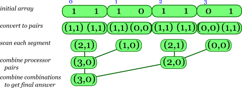
The parallel scan algorithm has some less obvious applications. Suppose we have an array of 0's and 1's, and we want to determine how many 1's begin the array. If our array were <1, 1, 1, 0, 1, 1, 0, 1>, we would want to determine that the array starts with three 1's.

You probably won't be able to imagine on your own some associative operator that we might use here. However, there is a common trick that we can apply, and with some practice you'll learn how to use this trick.

Our trick is to replace each element in the array with a pair. In this case, we'll change element a_i to become the pair (a_i, a_i) in our new array. We'll perform our scan on this new array of pairs using the ⊗ operator defined as follows:

(x, p) ⊗ (y, q) = (x + p y, p q)

To make sense of this, consider each pair to represent a segment of the array, with the first number saying how many 1's start the segment, while the second number is 1 or 0 depending on whether the segment consists entirely of 1's. When we combine two adjacent segments represented by the pairs (x, p) and (y, q), we first want to know the number of initial 1's in the combined segment. If p is 1, then the first segment consists entirely of x 1's, and so the total number of initial 1's in the combination includes these x 1's plus the y initial 1's of the second segment. But if p is 0, then the initial 1's in the combined segment lie entirely within the beginning of the first segment, where there are x 1's. The expression x + p y combines these two facts into one arithmetic expression. For the second part of the resulting pair, we observe that the combined segment consists of all 1's only if both segments consist of all 1's, and p q will compute 1 only if both p and q are both 1.

In order to know that our parallel scan algorithm works correctly, we must verify that our ⊗ operator is associative. We try both ways of associating (x, p) ⊗ (y, q) ⊗ (z, r) and see that they match.

((x, p) ⊗ (y, q)) ⊗ (z, r) = (x + p y, p q) ⊗ (z, r) = (x + p y + p q z, p q r)
(x, p) ⊗ ((y, q) ⊗ (z, r)) = (x, p) ⊗ (y + q z, q r)
= (x + p (y + q z), p q r) = (x + p y + p q z, p q r)

The following diagram illustrates how this would work for the array <1, 1, 1, 0, 1, 1, 0, 1> on four processors.

(A completely different approach to this problem — still using the parallel scan algorithm we've studied — is to change each 0 in the array to be its index within the array, while we change each 1 to be the array's length. Then we could use parallel scan to find the minimum element among these elements.)

2.4. Evaluating a polynomial

Here's another application that's not immediately obvious. Suppose we're given an array a of coefficients and a number x, and we want to compute the value of

a₀ ⋅ x^n − 1 + a₁ ⋅ x^n − 2 + … + a_n − 2 ⋅ x + a_n − 1.

Again, the solution isn't easy; we end up having to change each array element into a pair. In this case, each element a_i will become the pair (a_i, x). We then define our operator ⊗ as follows.

(p, y) ⊗ (q, z) = (p z + q, y z)

Where does this come from? It's a little difficult to understand at first, but each such pair is meant to summarize the essential knowledge needed for a segment of the array. This segment itself represents a polynomial. The first number in the pair is the value of the segment's polynomial evaluated for x, while the second is xⁿ, where n is the length of the represented segment.

But before we imagine using our parallel scan algorithm, we need first to confirm that the operator is indeed associative.

((a, x) ⊗ (b, y)) ⊗ (c, z) = (a y + b, x y) ⊗ (c, z)
= ((a y + b) z + c, x y z) = (a y z + b z + c, x y z)
(a, x) ⊗ ((b, y) ⊗ (c, z)) = (a, x) ⊗ (b z + c, y z) = (a y z + b z + c, x y z)

Both associations yield the same result, so the operator is associative. Let's look at an example to see it at work. Suppose we want to evaluate the polynomial x³ + x² + 1 when x is 2. In this case, the coefficients of the polynomial can be represented using the array <1, 1, 0, 1>. The first step of our algorithm is to convert this into an array of pairs.

(1, 2), (1, 2), (0, 2), (1, 2)

We can then repeatedly apply our ⊗ operator to arrive at our result.

(1, 2) ⊗ (1, 2) ⊗ (0, 2) ⊗ (1, 2)

= (1 ⋅ 2 + 1, 2 ⋅ 2) ⊗ (0, 2) ⊗ (1, 2) = (3, 4) ⊗ (0, 2) ⊗ (1, 2)

= (3 ⋅ 2 + 0, 4 ⋅ 2) ⊗ (1, 2) = (6, 8) ⊗ (1, 2)

= (6 ⋅ 2 + 1, 8 ⋅ 2) = (13, 16)

So we end up with (13, 16), which has the value we wanted to compute — 13 — as its first element: 2³ + 2² + 1 = 13.

In our computation above, we proceeded in left-to-right order as would be done on a single processor. In fact, though, our parallel scan algorithm would combine the first two elements and the second two elements in parallel:

(1, 2) ⊗ (1, 2) = (1 ⋅ 2 + 1, 2 ⋅ 2) = (3, 4)

(0, 2) ⊗ (1, 2) = (0 ⋅ 2 + 1, 2 ⋅ 2) = (1, 4)

And then it would combine these two results to arrive at (3 ⋅ 4 + 1, 4 ⋅ 4) = (13, 16).

3. Parallel prefix scan

Now we consider a slightly different problem: Given an array <a₀, a₁, a₂, …, a_n − 1>, we want to compute the sum of every possible prefix of the array:

<a₀, a₀ + a₁, a₀ + a₁ + a₂, …, a₀ + a₁ + a₂ + … + a_n − 1>

3.1. The prefix scan algorithm

This is easy enough to do on a single processor with code that takes O(n) time.

total = array[0]; for(i = 1; i < array.length; i++) { total += array[i]; array[i] = total; }

With p processors, we might hope to compute all prefix sums in O(n / p + log p) time, since we can find the sum in that amount of time. However, there's not a straightforward way to adapt our earlier algorithm to accomplish this. We can begin with an overall outline, though.

Each processor finds the sum of its segment.
total = segment[0]; for(i = 1; i < segment.length; i++) total += segment[i];
Somehow the processors communicate so that each processor knows the sum of all segments preceding it (excluding the processor's segment). Each processor will now call this sum total.
Now each processor updates the array elements in its segment to hold the prefix sums.
for(i = 0; i < segment.length; i++) { total += segment[i]; segment[i] = total; }

If we divide the array equally among the processors, then the first and last steps each take O(n / p) time. The hard part is step 2, which we haven't specified exactly yet. We know we have each processor imagining a number (the total for its segment), and we want each processor to know the sum of all numbers imagined by the preceding processors. We're hoping we can perform this in O(log p) time.

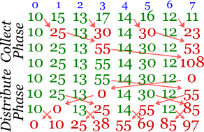
In 1990, parallel algorithms researcher Guy Blelloch described just such a technique. He imagined performing the computation in two phases, which we'll call the collect phase and the distribute phase, diagrammed below. (Blelloch called the phases up-sweep and down-sweep; these names make sense if you draw the diagrams upside-down from what I have drawn. You then have to imagine time as proceeding up the page.)


Collect Phase	Distribute Phase

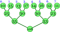
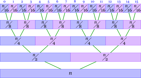
The collect phase is just like our parallel sum algorithm: Each starts with its segment's subtotal, and we have a binary tree that eventually sums these subtotals together. This takes log₂ p rounds of communication.

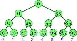
The distribute phase is more difficult. You can see that we start with 0, which that processor sends to its left. But the processor also sends 55 to its right — and where did the 55 come from? Notice that in the collect phase's tree 55 is the final node's left child. Similarly, the processor receiving the 55 in the first distribution round sends that to its left, and to the right it sends 85; it arrives at 85 by adding its left child from the collect phase, 30, onto the 55. At the same time, the processor that received 0 in the first distribution round sends 0 to its left child and 25 to its right; the 25 comes from adding its left child of 25 from the collect phase to the 0 it now holds.

While the tree may make sense, seeing exactly how to implement the distribute phase is a bit difficult at first. But the following diagram is quite helpful.

The first four rows represent the collect phase, just like the parallel sum from Section 2.1, except now the numbers are sent to the right, not the left. After the collect phase is finished, the final processor holds the overall total — but then it promptly replaces 108 with 0 before beginning the distribute phase. In the first round of the distribute phase, processors 3 and 7 perform something of a swap: Each processor sends the number it ended up with from the collect phase, with processor 7 adding what it receives (55) to what it previously held (0) to arrive at 55; processor 3 simply updates what it remembers to its received value, 0. In the next round, we perform the same sort of modified swap between processors 1 and 3 and between processors 5 and 7; in each case, the first processor in the pair simply accepts its received value, while the second processor adds its received value to what it held previously. By the last round, when all processors participate in the swap, each processor ends up with the sum of the numbers preceding it at the beginning.

You may well object that this is fine as long as the number of processors is a power of 2, but it doesn't address other numbers of processors. Indeed, it doesn't work unless p is a power of 2. If it isn't, then one simple solution is simply to round p down to the highest power of 2. There has to be a power of 2 between p / 2 and p, so we'll still end up using at least half of the available processors. In big-O bounds, we won't lose anything: Our algorithm takes O(n / p + log p) time when p is a power of 2; if we halve p (which would be the case where we lose the most processors), we end up at O(n / (p / 2) + log (p / 2)) = O(2 n / p + log p − log 2) = O(n / p + log p) just as before. It's a bit frustrating to simply ignore up to half of our processors, but most often it wouldn't be worth complicating our program, increasing the likelihood of errors and costing programmer time for the sake of a constant factor of 2.

And that brings us to actually writing some code implementing our algorithm.

// Note: Number of processors must be power of 2 for this to work correctly. // find sum of this processor's segment total = segment[0]; for(i = 1; i < segment.length; i++) total += segment[i]; // perform collect phase for(k = 1; k < procs; k *= 2) { if((pid & k) == 0) { send(pid + k, total); break; } else { total = receive(pid - k) + total; } } // perform distribute phase if(pid == procs - 1) total = 0; // reset last processor's subtotal to 0 if(k >= procs) k /= 2; while(k > 0) { if((pid & k) == 0) { send(pid + k, total); total = receive(pid + k); } else { int t = receive(pid - k); send(pid - k, total); total = t + total; } k /= 2; } // update array to have the prefix sums for(i = 0; i < segment.length; i++) { total += segment[i]; segment[i] = total; }

3.2. Filtering an array

Why would we ever want to find the sum for all prefixes of an array? This problem isn't quite as intuitive as wanting just the overall sum. But the algorithm still proves useful for several applications. One interesting application is filtering an array so that all elements satisfying a particular property are at its beginning. Below is code accomplishing this on a non-parallel machine, based on a pre-existing method named shouldKeep for determining whether a particular number satisfies the desired property.

int numKept = 0; for(int i = 0; i < arrayLength; i++) { if(shouldKeep(array[i])) { array[numKept] = array[i]; numKept++; } }

One example where we want to do this is during the pivot step of Quicksort: After selecting a pivot element, we want to move all elements that are less than this selected pivot to the beginning of the array (and all elements greater than the pivot to the end — but that is basically the same problem).

To accomplish our filtering, we first create another array where each entry is 1 if shouldKeep says to keep the corresponding element of the original array and 0 otherwise. Then we compute all prefix sums of this array. For each element that shouldKeep says to keep, the corresponding prefix sum indicates where it should be placed into the new array; so finally we can just place each kept number into the indicated index (minus 1).

For example, suppose we want to keep only the numbers ending in 3 or 7 in the array 2, 3, 5, 7, 11, 13, 17, 19. We compute the following values.

`input`:	2,	3,	5,	7,	11,	13,	17,	19
`keep`:	0,	1,	0,	1,	0,	1,	1,	0
`prefix`:	0,	1,	1,	2,	2,	3,	4,	4
`result`:	3,	7,	13,	17

The keep array is the result of testing whether each number ends in either 3 or 7. The prefix array holds the sum of each prefix of this array. And to compute result, we take each entry input_i where shouldKeep(input_i) is true, and we copy it into index prefix_i − 1.

3.3. Adding big integers

Just as we generalized our parallel sum algorithm from Section 2.1 to parallel scan in Section 2.2, we can also generalize our parallel prefix sum algorithm to work with an arbitrary operator ⊗. For this to work, our ⊗ operator must be associative — but it must also have an identity element: That is, there must be some value a for which a ⊗ x = x regardless of x. This identity is necessary for resetting the last processor's value as the distribute phase begins. In our work in Section 3.1, we reset the last processor's total to 0, since we were using addition for ⊗, and since 0 is the identity for addition.

We'll see an example of using a special definition for ⊗ by examining how to add two very large integers. Each big-integer is represented using an array <a₀, a₁, …, a_n − 2, a_n − 1> with each array entry representing one digit: a₀ is the big-integer's 1's digit, a₁ is its 10's digit, and so forth. We'll represent our second big-integer to add as <b₀, b₁, …, b_n − 2, b_n − 1> in the same format. We want to compute the sum of these two big-integers.

On a single-processor computer, we could accomplish this using the following code fragment.

carry = 0; for(i = 0; i < n; i++) { sum[i] = (a[i] + b[i] + carry) % 10; carry = (a[i] + b[i] + carry) / 10; }

Notice how this program uses the carry variable to hold a value that will be used in the next iteration. It's this carry variable that makes this code difficult to translate into an efficient program on multiple processors.

But here's what we can do: First, notice that our primary problem is determining whether each column has a carry for the next column. For determining this, we'll create a new array c, where each value is either C (for carry), M (for maybe), or N (for never). To determine entry c_i of this array, we'll compute a_i + b_i and assign c_i to be C if the sum is 10 or more (since in this case this column will certainly carry 1 into the following column), M if the sum is 9 (since this column may carry into the next column, if there is a carry from the previous column), and N if it is below 9 (since there is no possibility that this column will carry).

Now we'll do a parallel prefix scan on this c array with our ⊗ operator defined as in the below table.

`x`	`y`	`x` ⊗ `y`
N	N	N
N	M	N
N	C	C
M	N	N
M	M	M
M	C	C
C	N	N
C	M	C
C	C	C

More compactly, x ⊗ y is y if y is either C or N, but it is x if y is M. We can confirm that this ⊗ operator is associative by simply listing all 27 possible combinations for three variables x, y, and z and confirming that for each of them, (x ⊗ y) ⊗ z matches x ⊗ (y ⊗ z).

`x`	`y`	`z`	(`x` ⊗ `y`) ⊗ `z`	`x` ⊗ (`y` ⊗ `z`)
N	N	N	N	N
N	N	M	N	N
N	N	C	C	C
N	M	N	N	N
N	M	M	N	N
N	M	C	C	C
N	C	N	N	N
N	C	M	C	C
N	C	C	C	C

`x`	`y`	`z`	(`x` ⊗ `y`) ⊗ `z`	`x` ⊗ (`y` ⊗ `z`)
M	N	N	N	N
M	N	M	N	N
M	N	C	C	C
M	M	N	N	N
M	M	M	M	M
M	M	C	C	C
M	C	N	N	N
M	C	M	C	C
M	C	C	C	C

`x`	`y`	`z`	(`x` ⊗ `y`) ⊗ `z`	`x` ⊗ (`y` ⊗ `z`)
C	N	N	N	N
C	N	M	N	N
C	N	C	C	C
C	M	N	N	N
C	M	M	C	C
C	M	C	C	C
C	C	N	N	N
C	C	M	C	C
C	C	C	C	C

Moreover, we can see this operator has an identity because M ⊗ x is x regardless of x's value. Since our ⊗ operator is associative and has an identity, we can legimately use it for our prefix scan algorithm.

Let's see an example of how this might work. Suppose we want to add 13579 and 68123. These two five-digit numbers are represented with the arrays <9,7,5,3,1> and <3,2,1,8,6>. The steps we undertake to compute the sum are summarized in the table below.

a: < 9, 7, 5, 3, 1>

b: < 3, 2, 1, 8, 6>

c: < C, M, N, C, N>

prefix scan: < C, C, N, C, N>

carries: < 0, 1, 1, 0, 1>

sum: < 2, 0, 7, 1, 8>

`a`:	<	9,	7,	5,	3,	1>
`b`:	<	3,	2,	1,	8,	6>
`c`:	<	C,	M,	N,	C,	N>
prefix scan:	<	C,	C,	N,	C,	N>
carries:	<	0,	1,	1,	0,	1>
sum:	<	2,	0,	7,	1,	8>

We first compute the array c of C/M/N values based on summing corresponding columns from a and b; each column here is computed independently of the ohers, so c can be determined completely in parallel. We end up with <C,M,N,C,N>. Then we apply the parallel prefix scan algorithm on c using our ⊗ operator, arriving at <C,C,N,C,N>. Each entry c_i of this prefix scan indicates whether that column would carry into the following column. Thus, the carry into column i, which we term carry_i, will be 1 if entry c_i − 1 exists and is C, and otherwise carry_i will be 1. In our example, the carry array would be <0,1,1,0,1>. Our final step is to add corresponding columns of a, b, and carry, retaining only the 1's digit of each sum. In our example, we end up with <2,0,7,1,8>, corresponding to the result 81702.

4. Sorting

So far we have been working with very elementary problems — problems where the single-processor solution is so straightforward that in classical algorithms we rarely discuss the problems at all. Now we'll turn to one of the most heavily studied classical problems of all: sorting. How can we sort an array of numbers quickly when we have many processors?

We know we can sort an n-element array on a single processor in O(n log n) time. With p processors, then, we would hope to find an algorithm that takes O((n log n) / p) time. We won't quite achieve that here, but instead we'll look at an algorithm that takes O((n ((log p)² + log n) / p)) time. Our algorithm will be based on the mergesort algorithm. It's natural to look at mergesort, because it's a simple divide-and-conquer algorithm. Divide-and-conquer algorithms are particularly attractive for multiprocessor systems: After splitting the problem into subproblems, we split our processors to process each subproblem simultaneously, and then we need a way to use all our processors combine the subproblems' solutions together.

(Incidentally, there is a O((n log n) / p) algorithm for parallel sorting, developed in 1983 by Ajtai, Komlós, and Szemerédi and subsequently simplified by M. S. Paterson in 1990. Even the simplified version, though, is more complex than what we want to study here. What's more, the multiplicative constant hidden by the big-O notation turns out to be quite large — large enough to make it less efficient in the real world than the algorithm we'll study, which was developed by Ken Batcher in 1968.)

4.1. Merging

Our first problem is determining how to merge two arrays of similar length. For the moment, we'll imagine that we have as many processors as we have array elements. Below is a diagram of how to merge two segments, each with 8 elements.

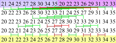
The first round here consists of comparing the elements of each sorted half with the element at the same index in the other sorted half; and for each pair, we will swap the numbers if the second number is less than the first. Thus, the 21 and 20 are compared, and since 20 is less, it is moved into the processor 0, while the 21 moves up to processor 8. At the same time, processors 1 and 9 compare 24 and 22, and since they are out of order, these numbers are swapped. Note, though, that the 28 and 31 are compared but not moved, since the lesser is already at the smaller-index processor.

The second round of the above diagram involves several comparisons between processors that are 4 apart. And the third round involves comparisons between processors that are 2 apart, and finally there are comparisons between adjacent processors.

We've illustrated the process with a single number for each processor. In fact, each processor will actually have a whole segment of data. Where our above diagram indicates that two processors should compare numbers, what will actually happen is that the two processors will communicate their respective segments to each other and each will merge the two segments together. The lower-index processor keeps the lower half of the merged result, while the upper-index processor keeps the upper half.

Below is some pseudocode showing how this might be implemented. In order to facilitate its usage in mergesort later, this pseudocode is written imagining that only a subset of the processors contain the two arrays to be merged.

void merge(int firstPid, int numProcs) { // Note: numProcs must be a power of 2, and firstPid must be a multiple of // numProcs. The numProcs / 2 processors starting from firstPid should hold one // sorted array, while the next numProcs / 2 processors hold the other. int d = numProcs / 2; if(pid < firstPid + d) mergeFirst(pid + d); else mergeSecond(pid - d); while(d >= 2) { d /= 2; if((pid & d) != 0) { if(pid + d < firstPid + numProcs) mergeFirst(pid + d); } else { if(pid - d >= firstPid) mergeSecond(pid - d); } } } void mergeFirst(int otherPid) { send(otherPid, segment); // send my segment to partner otherSegment = receive(otherPid); // receive partner's whole segment merge segment and otherSegment, keeping the first half in my segment variable; } void mergeSecond(int otherPid) { otherSegment = receive(otherPid); // receive partner's whole segment send(otherPid, segment); // send my segment to partner merge segment and otherSegment, keeping the second half in my segment variable; }

Though the algorithm may make sense enough, it isn't at all obvious that it actually is guaranteed always to merge the two halves into one sorted array. The argument that it works is fairly involved, and we won't go into it here.

We will, though, examine how much time the algorithm takes. Since with each round the involved processors will send, receive, and merge segments of length ⌈n / p⌉, each round of our algorithm will take O(n / p) time. Because there are log₂ p rounds, the total time taken to merge both arrays is O((n / p) log p).

4.2. Mergesort

Now we know how to merge two (n / 2)-length arrays on p processors in O((n / p) log p) time. How can we use this merging algorithm to sort an array with n elements?

Before we can perform any sorting, we must first sort each individual processor's segment. You've studied single-processor sorting thoroughly before; we might as well use the quicksort algorithm here. Each processor has ⌈n / p⌉ elements in its segment, so each processor will take O((n / p) log (n / p)) = O((n / p) log n) time. All processors perform this quicksort simultaneously.

Now we will progressively merge sorted segments together, until the entire array is one large sorted segment, as diagrammed below.

This is accomplished using the following pseudocode, which uses the merge subroutine we developed in Section 4.1.

void mergeSort() { perform quicksort on my segment; int sortedProcs = 1; while(sortedProcs < procs) { sortedProcs *= 2; merge(pid & ~(sortedProcs - 1), sortedProcs); } }

Let's continue our speed analysis by skipping to thinking about the final level of our diagram. For this last level, we have two halves of the array to merge, with n elements between them. We've already seen that merging these halves takes O((n / p) log p) time. Removing the big-O notation, this means that there is some constant c for which the time taken is at most c ((n / p) log p).

Now we'll consider the next-to-last level of our diagram. Here, we have two merges happening simultaneously, each taking two sorted arrays with a total of n / 2 elements. Half of our processors are working on each merge, so each merge takes at most c (((n / 2) / (p / 2)) log (p / 2)) = c ((n / p) log (p / 2)) ≤ c ((n / p) log p) time — the same bound we arrived at for the final level. That is the time taken for each of the two merges at this next-to-last level; but since each merge is occurring simultaneously on a different set of processors, it is also the total time taken for both merges.

Similarly, at the third-from-last level, we have four simultaneous merges, each performed by p / 4 processors merging two sorted arrays with a total of n / 4 elements. The time taken for each such merge is c (((n / 4) / (p / 4)) log (p / 4)) = c ((n / p) log (p / 4)) ≤ c ((n / p) log p). Again, because the merges occur simultaneously on different sets of processors, this is also the total time taken for this level of our diagram.

What we've seen is that for each of the last three levels of the diagram, the time taken is at most c((n / p) log p). Identical arguments will work for all other levels of the diagram except the first. There are log₂ p such levels, each being performed after the previous one is complete. Thus the total time taken for all levels but the first is at most (c ((n / p) log p)) log₂ p = O((n / p) (log p)²).

We've already seen that the first level — where each processor independently sorts its own segment — takes O((n / p) log n) time. Adding this in, we arrive at our total bound for mergesort of O((n / p) ((log p)² + log n)).

5. Hardness of parallelization

For many problems, we know of a good single-processor algorithm, but there seems to be no way to adapt the algorithm to make good use of additional processors. A natural question to ask is whether there really is no good way to use additional processors. After all, if we can't prove that efficient parallelization is impossible, how can we know when to stop trying?

There is no known technique for addressing this question perfectly. However, there is an important partial answer worth studying. This answer uses complexity theory, the same field where people study the class P, which includes problems that can be solved in polynomial time, and NP, which includes many more problems, including many that people have studied intensively for decades without finding any polynomial-time solution. Some of these difficult problems within NP have been proven to be NP-complete, which means that finding a polynomial-time algorithm for that problem would imply that all problems in NP can also be solved in polynomial time. Since it's unlikely that all those well-studied problems have polynomial-time algorithms, a proof that a problem is NP-complete is tantamount to an argument that one can't hope for a polynomial-time algorithm solving it.

To discuss parallelizability in the context of complexity theory, we begin by defining a new class of problems called NC. (The name is quite informal: It stand's for Nick's Class, after Nick Pippenger, a complexity researcher who studied some problems related to parallel algorithms.) This class includes all problems for which an algorithm can be constructed with a time bound that is polylogarithmic in n (i.e., O((log n)^d) for some constant d, where n is the size of the problem input) if given a number of processors polynomial in n.

An example of a problem that is in NC is adding two big-integers together. We've seen that this problem can be solved with p processors in O(n / p + log p) time. This isn't itself polylogarithmic in n, but suppose we happened to have n processors. This is of course a polynomial number of processors, and the amount of time taken would be O(1 + log n) = O(log n), which is polylogarithmic in n. For this reason, we know that adding big-integers is in NC.

What about sorting? In Section 4 we saw an O((n / p) ((log p)² + log n)) algorithm. Again, suppose the number of processors were n, which is of course a polynomial in n. In that case, the time taken could be simplified to O((log n)² + log n) = O((log n)²), which again is polylogarithmic in n. We can conclude that sorting is also within NC.

Just as with P and NP we naturally ask what the relationship is between P and NC. One thing that is easy to see is that any problem within NC is also within P: After all, we can simulate all p processors on just a single processor, which ends up multiplying the time taken by p. But since p must be a polynomial in n and we're multiplying this polynomial by a polylogarithmic time for each processor, we'll end up with a polynomial amount of time.

But what is much harder to see is whether every problem within P is also in NC — that is, whether every problem that admits a polynomial-time solution on a single processor can be sped up to take polylogarithmic time if we were given a polynomial number of processors. Nobody has been able to show one way or another whether any such problems exist. In fact, the situation is quite analogous to that between P and NP: Technically, nobody has proven that there is a P problem that definitely is not within NC — but there are many P problems for which people have worked quite hard to find polylogarithmic-time algorithms using a polynomial number of processors: Surely at least one of these problems isn't in NC!

People have been able to show, though, that there are some problems that are P-complete: That is, if the P-complete problem could be shown to be within NC, then in fact all problems within P lie within NC. (Here, we're talking about P-completeness with respect to NC. For our purposes, this is a minor technicality; it's only significant when you study some of the other complexity classes below P.) Since many decades of research indicate that the last point isn't true, we can't reasonably hope to find a polylogarithmic-time solution to a P-complete problem.

While we won't look rigorously at how one demonstrates P-completeness, we can at least look briefly at a list of some problems that have been shown to be P-complete.

Given a circuit of AND and OR gates and the inputs into the circuit, compute the output of the circuit.
Compute the preorder number for a depth-first search of a dag.
Compute the maximum flow of a weighted graph.

Knowing that a problem is P-complete doesn't really mean that additional processors will never help. For instance, a graph's maximum flow can be computed in O(m² n) time using the Ford-Fulkerson algorithm. (And it happens there's a more complex algorithm that takes O(m n log (n² / m)) time.) However, with many processors, we could still hope to find an O(m² n / p + √p) algorithm without making any major breakthroughs in the NC = P question.

Still, knowing about P-completeness gives us some limits on how much we can hope for from multiple processors. Usually parallel and distributed systems can provide significant speedup. But not always. And, as we've seen, the algorithm providing the speedup is often much less obvious than the single-processor algorithm.

Review questions

Distinguish between a parallel system and a distributed system.
Without referring explicitly to our parallel sum or parallel scan algorithms, describe how a parallel-processor system with p processors can compute the minimum element of an n-element array in O(n / p + log p) time. You may assume that each processor has an ID between 0 and p − 1.
Given an array <a₀, a₁, …, a_n − 1> and some associative operator ⊗, describe what the parallel prefix scan algorithm computes.
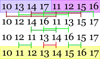
Section 4.1 includes a diagram illustrating the comparisons made as a 16-processor system merges two 8-element arrays. Draw a similar diagram demonstrating the comparisons made for merging the two arrays <10, 13, 14, 17> and <11, 12, 15, 16>.
What does it mean for a problem to be in the NC complexity class? Give an example of a problem that is P-complete and so is probably not amenable to radical improvements in running time using multiple processors.
Suppose we're working on a problem where n is the number of bits in the problem input and p is the number of processors. We develop an algorithm whose time requirement is
O(n²/√p + (log p)²) .
Can we conclude that this problem is in the NC complexity class? Explain why or why not.

Solutions to review questions

Both involve multiple processors. However, in a parallel system we assume that communication between processors is very cheap, and communication is usually through shared access to the same memory. But in distributed systems, we assume the processors are somewhat separated, without any shared memory, and communication occurs through passing messages across a local network — quite a bit more expensive than accessing shared memory.
Each processor computes the minimum of its segment of the array. This takes O(n / p) time.

Now each processor whose ID is odd sends its minimum to the one before it, which determines which is the smaller of its segment's minimum and the other processor's minimum. That represents the minimum of both processors' segments. Since there is just one message being sent or received by each processor, this takes O(1) time.

And then each processor whose ID is even but not a multiple of 4 sends its minimum to the multiple of 4 before it, and that processor determines which is the smaller of that number what what it thought was the minimum before. As a result, each processor with an ID that is a multiple of 4 will now know the smallest value in four processors' segments. Again, this step takes O(1) time.

We repeat the process, each time halving the number of active processors (that is, ones that received a message in the last step and will continue working in the next step). When there is just one active processor, we stop. There will be ⌈log₂ p⌉ such rounds, each taking O(1) time, so the combination of the segments' minima takes a total of O(log p) time.
It computes the array: <a₀, a₀ ⊗ a₁, a₀ ⊗ a₁ ⊗ a₂, …, a₀ ⊗ a₁ ⊗ a₂ ⊗ … ⊗ a_n − 1>.
A problem is in NC if an algorithm for it exists that, given a number of processors polynomial in n (the size of the problem input), can compute the answer in time polylogarithmic in n (i.e., O((log n)^d) for some constant d).

Examples of P-complete problems cited in Section 5 include:
- Given a circuit of AND and OR gates and the inputs into the circuit, compute the output of the circuit.
- Compute the preorder number for a depth-first search of a dag.
- Compute the maximum flow of a weighted graph.
Yes, it is in NC. After all, if we had n⁴ processors, our algorithm would take O((n² / √n⁴) + (log n⁴)²) = O((n² / n²) + (4 log n)²) = O(1 + 16 (log n)²) = O((log n)²) time. The number of processors in this case would be polynomial, while the time taken would be polylogarithmic, as required for NC.

Exercises

At the end of Section 2.1 we saw some code that performs a parallel scan in O(n / p + log p) time. That code was written using the message-passing methods described in Section 1.2. Adapt the code to instead fit into a shared-memory system of Section 1.1. For synchronization, you should assume that there is an array named signals containing p objects; each object supports the following two methods.

void set()

Marks this object as being set. The object defaults to being unset.. Setting the object will awaken anybody who is waiting in the waitUntilSet method.

void waitUntilSet()

Returns once this object is set. This could return immediately if this object has already been set; otherwise, the method will delay indefinitely until somebody sets this object.

Suppose we're given an array of pairs (a_i, b_i), where a₀ is 0. This array of pairs specifies a sequence of linear equations as follows:

`x`₀	=	`b`₀
`x`₁	=	`a`₁ `x`₀ + `b`₁
`x`₂	=	`a`₂ `x`₁ + `b`₂
	:	(and so forth)

We want to compute x_n − 1. We could do this easily enough on a single-processor system.

double x = b[0]; for(int i = 1; i < n; i++) x = a[i] * x + b[i];

But we have a parallel system and wish to compute the final answer more quickly. A natural approach is to try to adapt our parallel scan operation using an operator ⊗ as follows.

(a, b) ⊗ (a′, b′) = (0, a′ b + b′)

Applying this ⊗ operator left-to-right through the array, we see that we end up with the appropriate values for each x (recalling that a₀ is defined to be 0).

(0, `b`₀) ⊗ (`a`₁, `b`₁)	=	(0, `a`₁ `b`₀ + `b`₁)	=	(0, `x`₁)
(0, `x`₁) ⊗ (`a`₂, `b`₂)	=	(0, `a`₂ `x`₁ + `b`₂)	=	(0, `x`₂)
(0, `x`₂) ⊗ (`a`₃, `b`₃)	=	(0, `a`₃ `x`₂ + `b`₃)	=	(0, `x`₃)
		:

Unfortunately, we can't apply the parallel scan algorithm to this operator because it isn't associative.

((`a`, `b`) ⊗ (`a`′, `b`′)) ⊗ (`a`″, `b`″)		=	(0, `a`′ `b` + `b`′) ⊗ (`a`″, `b`″)
=	(0, `a`″ (`a`′ `b` + `b`′) + `b`″)	=	(0, `a`″ `a`′ `b` + `a`″ `b`′ + `b`″)
(`a`, `b`) ⊗ ((`a`′, `b`′) ⊗ (`a`″, `b`″))		=	(`a`, `b`) ⊗ (0, `a`″ `b`′ + `b`″)
=	(0, 0 `b` + (`a`″ `b`′ + `b`″))	=	(0, `a`″ `b`′ + `b`″)

Show a new definition of ⊗ — a slight modification of the one shown above — which is associative and yields the correct value of x_n − 1 when applied to our array.

Suppose we have an array of opening and closing parentheses, and we want to know whether the parentheses match — that is, we consider (()())() to match, but not )(())()( or (()))((). Using the parallel scan and/or parallel prefix scan operations, show how to determine this in O(n / p + log p) on a p-processor system. (You need not define a novel ⊗ operator unless it suits your purpose.)
Suppose we're given an n-element array of (θ, d) pairs, representing a sequence of commands to a turtle to turn counterclockwise θ degrees and then go forward d units. Below is an example array and the corresponding movement it represents, where the turtle's initial orientation is to the east — though the first command immediately turns the turtle to face northeast.

array of commands movement diagram

0: (45, 40)

1: (30, 50)

2: (105, 40)

3: (90, 20)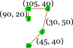

Suppose we have a p-processor system, and we want to compute the turtle's final location in O(n / p + log p) time. Describe such an algorithm using the parallel scan and/or parallel prefix scan algorithms. Argue briefly that your algorithm works correctly.
On a parallel system, we have an array of messages represented as integers and an array saying how far each message should be copied into the array. For example, given the two arrays msgs and dist below, we want to arrive at the solution recv.

0 1 2 3 4 5 6 7 8

msgs 3, 0, 0, 8, 0, 0, 5, 6, 0

dist 3, 0, 0, 2, 0, 0, 1, 2, 0

recv 3, 3, 3, 8, 8, 0, 5, 6, 6

In this example, dist[0] is 3, and so we see that msgs[0] occurs in the three entries of recv starting at index 0. Similarly, dist[7] is 2, so msgs[7] is copied into the two entries of recv starting at index 7. You may assume that dist is structured so that no interval overlaps (for example, if dist[0] is 4, then dist[1] through dist[3] will necessarily be 0) and the final interval does not go off the array's end. However, there may be some entries that lie outside any interval — as you can see with entry 5 in the above example.

Show how this job can be accomplished using a parallel prefix scan. This is a matter of identifying an operation ⊗, explaining why you know this operator does its job, and showing that the operator is associative and has an identity.

	0	1	2	3	4	5	6	7	8
`msgs`	3,	0,	0,	8,	0,	0,	5,	6,	0
`dist`	3,	0,	0,	2,	0,	0,	1,	2,	0
`recv`	3,	3,	3,	8,	8,	0,	5,	6,	6

References

Guy Blelloch, Prefix Sums and Their Applications, in Synthesis of Parallel Algorithms, edited by John H Reif, Morgan Kaufmann, 1991.: This book chapter introduces the parallel scan as a computation primitive. The book is hard to find, but you can freely download the chapter from the author's Web site.
Alan Gibbons and Wojciech Rytter, Efficient Parallel Algorithms, Cambridge University Press, 1989.: This short book (268 pages) is a good survey of parallel algorithms, though it is a bit dated. It includes a discussion of parallel sorting algorithms and P-completeness.
Mark Harris, Shubhabrata Sengupta, and John Owens, Parallel Prefix Sum (Scan) with CUDA, in GPU Gems 3, edited by Hubert Nguyen, 2007.: The article is for programmers trying to learn CUDA, a toolkit developed by NVIDIA for writing programs for execution on their GPUs.
Robert Sedgewick, Algorithms in Java, Parts 1–4, Addison-Wesley, 2002.: This book includes a more extensive discussion of Batcher's sorting algorithm, with an argument for why it works.

((`x`, `p`) ⊗ (`y`, `q`)) ⊗ (`z`, `r`)	= (`x` + `p` `y`, `p` `q`) ⊗ (`z`, `r`)	= (`x` + `p` `y` + `p` `q` `z`, `p` `q` `r`)
(`x`, `p`) ⊗ ((`y`, `q`) ⊗ (`z`, `r`))	= (`x`, `p`) ⊗ (`y` + `q` `z`, `q` `r`)
	= (`x` + `p` (`y` + `q` `z`), `p` `q` `r`)	= (`x` + `p` `y` + `p` `q` `z`, `p` `q` `r`)

((`a`, `x`) ⊗ (`b`, `y`)) ⊗ (`c`, `z`)	= (`a` `y` + `b`, `x` `y`) ⊗ (`c`, `z`)
	= ((`a` `y` + `b`) `z` + `c`, `x` `y` `z`)	= (`a` `y` `z` + `b` `z` + `c`, `x` `y` `z`)
(`a`, `x`) ⊗ ((`b`, `y`) ⊗ (`c`, `z`))	= (`a`, `x`) ⊗ (`b` `z` + `c`, `y` `z`)	= (`a` `y` `z` + `b` `z` + `c`, `x` `y` `z`)

(1, 2) ⊗ (1, 2) ⊗ (0, 2) ⊗ (1, 2)
	=	(1 ⋅ 2 + 1, 2 ⋅ 2) ⊗ (0, 2) ⊗ (1, 2)	=	(3, 4) ⊗ (0, 2) ⊗ (1, 2)
	=	(3 ⋅ 2 + 0, 4 ⋅ 2) ⊗ (1, 2)	=	(6, 8) ⊗ (1, 2)
	=	(6 ⋅ 2 + 1, 8 ⋅ 2)	=	(13, 16)

(1, 2) ⊗ (1, 2)	=	(1 ⋅ 2 + 1, 2 ⋅ 2)	=	(3, 4)
(0, 2) ⊗ (1, 2)	=	(0 ⋅ 2 + 1, 2 ⋅ 2)	=	(1, 4)