Recursion on integers is similar to recursion on sequences. Typically you have a base case — maybe when the integer is 0 or 1 — and the recursive case makes recursive calls to smaller integers than our parameter.
Computing factorials is a typical example. Recall that the factorial of an integer n is the product of all the integers from 1 to n. For example, the factorial of 5 is 120, from 1 ⋅ 2 ⋅ 3 ⋅ 4 ⋅ 5.
To compute factorials recursively, we might have our base case being when the parameter value is 1. For the recursive case, we compute the previous factorial — to get the product of the integers up to n − 1 — and then we can multiply that by n to get the next factorial.
def factorial(n):

    if n <= 1:

        return 1

    else:

        prev = factorial(n - 1)

        return prev * n
A more complex example of recursion is Fibonacci numbers. This is an infinite sequence of integers starting with 1 and 1, and where each succeeding number is the sum of the two preceding numbers in the sequence.
1, 1, 2, 3, 5, 8, 13, 21, 34, 55, 89, 144, …
Now suppose we want a function that takes some index and is supposed to return the Fibonacci number at that index. For example, given the index 7, we would hope to return 21, since if you go through the sequence indexing from 0, you would find that 21 is at position 7 in the sequence.
We can do this recursively as follows.
def fib(index):

    if index <= 1:

        return 1

    else:

        a = fib(index - 2)

        b = fib(index - 1)

        return a + b
Notice that this is a bit different from our examples so far, because the recursive case actually involves two recursive calls. This will make tracing through what happens quite a bit more complex.
For example, suppose we want to compute fib(5).
Here are the steps the computer goes through to compute the
value.
fib(5). Since 5 > 1, we
enter the else.fib(3).
fib(3). Since 3 > 1, we
enter the else.fib(1).
fib(1). Since 1 ≤ 1,
we immediately return 1 as our result.fib(1), 1, is stored in a.
We now must compute fib(2).
fib(2). Since 2 > 1, we
enter the else.fib(0).
fib(0). Since 0 ≤ 1,
we immediately return 1 as our result.fib(0), 1, is stored in a.
We now must compute fib(1).
fib(1). Since 1 ≤ 1,
we immediately return 1 as our result.b.
We add a and b, which is 2, and return this as
our result.b.
We add a and b, which is 3, and return this as
our result.fib(3), 3, is stored in a.
We now must compute fib(4).
fib(4). Since 4 > 1, we
enter the else.fib(2).
fib(2). Since 2 > 1, we
enter the else.fib(0).
fib(0). Since 0 ≤ 1,
we immediately return 1 as our result.fib(0), 1, is stored in a.
We now must compute fib(1).
fib(1). Since 1 ≤ 1,
we immediately return 1 as our result.b.
We add a and b, which is 2, and return this as
our result.fib(2), 2, is stored in a.
We now must compute fib(3).
fib(3). Since 3 > 1, we
enter the else.fib(1).
fib(1). Since 1 ≤ 1,
we immediately return 1 as our result.fib(1), 1, is stored in a.
We now must compute fib(2).
fib(2). Since 2 > 1, we
enter the else.fib(0).
fib(0). Since 0 ≤ 1,
we immediately return 1 as our result.fib(0), 1, is stored in a.
We now must compute fib(1).
fib(1). Since 1 ≤ 1,
we immediately return 1 as our result.b.
We add a and b, which is 2, and return this as
our result.b.
We add a and b, which is 3, and return this as
our result.b.
We add a and b, which is 5, and return this as
our result.b.
We add a and b, which is 8, and return this as
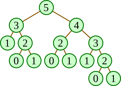
our result.Since the recursion process can get fairly complex, it can be useful to have a diagram of all the recursive calls. A recursion tree accomplishes this: Each node in the tree corresponds to a recursive call, where the nodes connected to it below are recursive calls made by that node.
Here's the recursion tree diagramming what happens in
computing fib(5).
As an example, you can see that the node labeled 4 in this tree has two
nodes below it, labeled 2 and 3. This is because in computing
fib(4), there are two recursive calls, one with an
argument of 2 and another with an argument of 3.
Naturally, any base cases have no nodes below them, since there are no recursive calls in a base case. Thus, there is nothing below any node labeled 0 or 1 in the recursion tree.